Datei:NumInt-MC.png

Größe dieser Vorschau: 800 × 600 Pixel. Weitere Auflösungen: 320 × 240 Pixel | 640 × 480 Pixel | 1.024 × 768 Pixel | 1.200 × 900 Pixel.
Originaldatei (1.200 × 900 Pixel, Dateigröße: 16 KB, MIME-Typ: image/png)
Beschreibung
| Beschreibung |
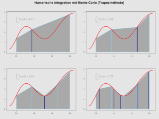
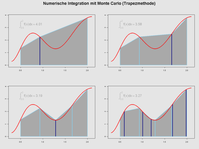
English: numerical intergration with monte carlo. new points are dark blue (navy), old points are skyblue. points/nodes are uniform distributed over the integration interval. the value of the integral tends to 3,32. |
| Datum | |
| Quelle | created with the help of GNU R, see source below |
| Urheber | Thomas Steiner |
| Genehmigung (Weiternutzung dieser Datei) |
Thomas Steiner put it under the GFDL |
Source code
R-source code:
 a=0.5
 b=2
 cs=c("red","skyblue","navy","darkgrey")

 f<-function(x) {
   return( 0.9*sin(9*x^0.6+0.3)+x+0.9 )
 }

 mc_plot<-function(n,new=1) {
   set.seed(6911)
   x=seq(a*0.6,b*1.05,length=700)
   if (n>0) {
     xi=sort((b-a)*runif(n)+a)
   } else {
     xi=NA
   }
   Xi=sort((b-a)*runif(new)+a)
   pts=sort(c(a,xi,Xi,b))
   plot(x,f(x),type="n",ylim=range(f(x),0),xlab="",ylab="")
   polygon(c(pts,b,a),c(f(pts),0,0),col=cs[4], border=cs[2],lwd=2)
   for (i in xi) {
     segments(i,0,i,f(i),col=cs[2],lwd=3)
   }
   for (i in Xi) {
     segments(i,0,i,f(i),col=cs[3],lwd=3)
   }
   lines(x,f(x),col=cs[1],lwd=3)
   ##calcualte area (integral)
   area=0
   for (p in 1:(length(pts)-1) ) {
     area <- area + (pts[p+1]-pts[p]) * (f(pts[p+1])+f(pts[p])) / 2
   }
   text(x=0.45,y=3.2, labels=substitute(integral(f(x)*dx, A, B)%~~% AREA,list(A=a,B=b,AREA=format(area,digits=3))),cex=1.5,col=cs[4],pos=4)
 }


 png(filename = "NumInt-MC.png", width=1200, height=900, pointsize = 12)
 par(bg="grey90",mfrow=c(2,2), oma=c(0,0,3,0), cex.axis=0.85)
 mc_plot(n=0)
 mc_plot(n=1)
 mc_plot(n=2)
 mc_plot(n=3,new=5)
 title(main="Numerische Integration mit Monte Carlo (Trapezmethode)", outer=TRUE,cex.main=1.9)
 dev.off()

|
Es ist erlaubt, die Datei unter den Bedingungen der GNU-Lizenz für freie Dokumentation, Version 1.2 oder einer späteren Version, veröffentlicht von der Free Software Foundation, zu kopieren, zu verbreiten und/oder zu modifizieren; es gibt keine unveränderlichen Abschnitte, keinen vorderen und keinen hinteren Umschlagtext.
Der vollständige Text der Lizenz ist im Kapitel GNU-Lizenz für freie Dokumentation verfügbar. |
| Diese Datei ist unter der Creative-Commons-Lizenz „Namensnennung – Weitergabe unter gleichen Bedingungen 3.0 nicht portiert“ lizenziert. | ||
| ||
| Diese Lizenzmarkierung wurde auf Grund der GFDL-Lizenzaktualisierung hinzugefügt. |
Dateiversionen
Klicke auf einen Zeitpunkt, um diese Version zu laden.
| Version vom | Vorschaubild | Maße | Benutzer | Kommentar | |
|---|---|---|---|---|---|
| aktuell | 15:13, 13. Apr. 2006 | | 1.200 × 900 (16 KB) | wikimediacommons>Thire | {{Information| |Description = numerical intergration with monte carlo. new points are dark blue (navy), old points are skyblue |Source = created with the help of GNU R, see source below |Date = 13 Apr. 2006 |Author = Thomas Steiner |
Dateiverwendung
Die folgende Seite verwendet diese Datei: